
A tutorial on Genome-Wide Association Studies (GWAS) in Tassel (GUI)
Updated:
Genome-wide association studies (GWAS) increase their popularity among medical, biological, and social sciences to identify the association between single nucleotide polymorphisms and phenotypic traits. This tutorial aims to provide a guidelines for conducing genome wide analysis in Tassel.
TASSEL
TASSEL also known as for the Evaluate traits aSSociations, Evolutionary Patterns, and linkage disequilibrium. It is a powerful statistical software to conduct association mapping such as General Linear Model (GLM) and Mixed Linear Model (MLM). The Tassel has ability to handle a wide range of indels (insertion & deletions).
The GUI (graphical user interface) version of TASSEL is very well built for anyone who does not have a background or experience in working in command line. I will show how to prepare input files and run association analysis in TASSEL. For detailed information on TASSEL, user’s guide and further documentation please visit: https://www.maizegenetics.net/tassel
1.0 Download and install TASSEL software
Download and install the latest version of the TASSEL software at this link: https://www.maizegenetics.net/tassel
1.1: Preparing the Input files
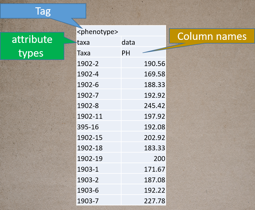
Phenotype file
Prepare the phenotype file as shown below in the figure, and please remember if your data has covariates such as sex, age or treatment, then, please categories them with header name factor.
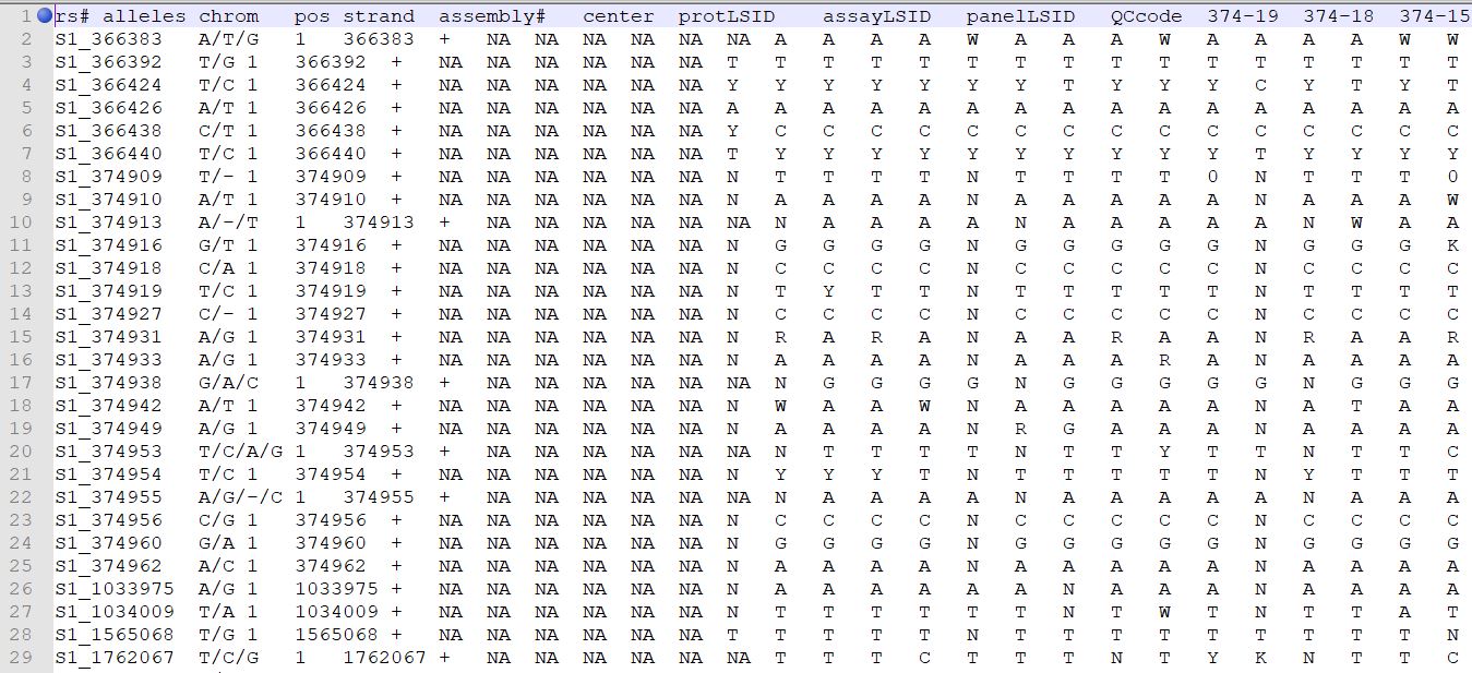
Genotype file
TASSEL allows various genotype file formats such as VCF (variant call format), .hmp.txt, and plink. In this tutorial, I am using the hmp.txt version of the genotype file. The below githe screenshot of the hmp.txt genotype file.
1.2: Importing phenotype and genotype files
Import the files by following the steps shown below.
Tip! Both files can be opened at same time holding
CTRLand clicking the file names.
1.3 Checking data on the basis of Phenotype distribution plot
It is always a wise idea to look at the phenotype distribution by plotting to check for any outliers. Follow below steps to plot histogram of your phenotype data.
1.5 Genotype summary analysis
Next crucial step is to look at the genotype data by simply following the steps shown. Couple of keys things to look at are:
- Minor allele frequency distribution
- Missing genotypic data to see if it requires to be imputed
- Proportion of heterozygous in the samples to check for self-ed samples
2.0 Conduct GWAS analysis
2.1 multidimensional scaling (MDS)
MDS output can be used as the covariate in the GLM or MLM to correct for population structure. Please follow the steps shown below:
2.2 Intersecting the files
Intersect the genotype, phenotype and MDS files by following the steps below:
3.0 running General Linear Model (GLM)
Run the GLM analysis by selecting the intersected files following the steps below:
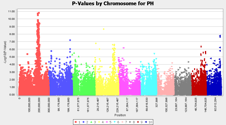
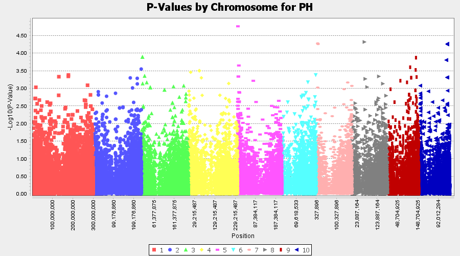
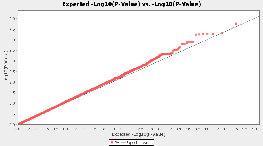
The output of the GLM analysis is produced under the Result node. The GLM association test can be evaluated by plotting Q-Q plot and the Manhattan plot as shown below.
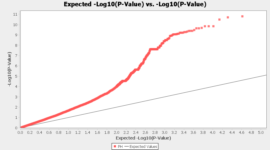
From the above Q-Q plot, we can see that are several markers that appear to be falsely associated with the trait, therefore, to control this confounding effect, use Kinship matrix as an another covariate in the linear model
4.0 Mixed Linear Model (MLM)
Mixed Linear Model used Unified Mixed-Model Method for Association Mapping. It helps to reduces Type I error in association mapping with complex pedigrees, families, founding effects and population structure.
4.1 Calculating Kinship matrix
Follow the below steps to calculate the kinship matrix:
4.2 running Mixed Linear Model (MLM)
MLM model includes the PCA and the kinship matrix i.e. MLM(PCA+K).
Therefore, once the Kinship matrix has been calculated, MLM can be now be conducted by following below steps:
Plot the output (MLM stats file in the Results branch following the above shown steps).
4.2 Exporting results
One may export the results in .txt format by the following the below steps:
4.3 Significance Threshold
Bonferroni threshold can be determined to identify significantly markers associated with the trait by using the below equation:
P ≤ 1/N (α =0.05)
where, N is the total number of markers tested in association analysis) was used to identify the most significantly markers associated with the trait. Similarly, another way is to perform FDR (False Discovery Rate) correction method.
Thank you for reading this tutorial. If you have any query or comments, please let me know in the comment section below or send me an email.
Bibliography
Bradbury PJ, Zhang Z, Kroon DE, Casstevens TM, Ramdoss Y, Buckler ES. (2007) TASSEL: Software for association mapping of complex traits in diverse samples. Bioinformatics 23:2633-2635.
Yu, J., Pressoir, G., Briggs, W. et al. (2006) A unified mixed-model method for association mapping that accounts for multiple levels of relatedness Nat Genet 38, 203–208. https://doi.org/10.1038/ng1702
Leave a comment