Investigate genetic admixture using STRUCTURE software
Updated:
Structure Software is a freely available software package that one may use for rigorous investigation of admixed individuals; identification of point of hybridization and migrants; and estimate over all structure of a population using commonly used genetic markers such as single nucleotide polymorphism (SNPs) and simple sequence repeat (SSRs).
This software was developed by Pritchard Lab at Stanford University and can be downloaded at this link.
Download sample data set: click here
In this tutorial, I will show how to prepare input files and run the Structure software. For detail information, please read this article at this link.
Step 1: Preparing the Input File
In this tutorial, I am using numerical SNP data as an input genotype file. One can convert their genotype data in numerical format in TASSEL software or any software package available as per one’s convenience. The file needs to be formatted properly as shown in the image below and saved as a .txt file.
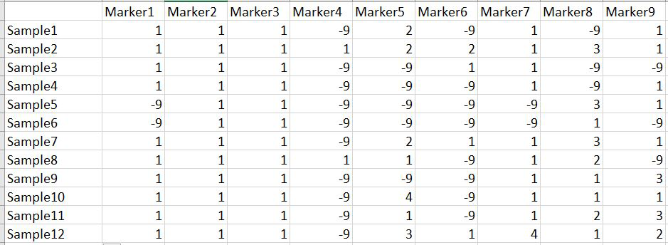
Please Note: Missing data is denoted as
-9in the above image.
Step 2: Running the Structure Software
Step 1.1: Importing the Input File
Once the input file with the correct header and format is ready, import the file in Structure software using the steps shown in the figure below. The importing process includes 4 steps — please make sure to select the correct directory and file name. At step 2 of 4, make sure to correctly input the number of markers, samples/individual, and ploidy (if genotypes are A enter 1; if AA enter 2), and finally indicate how missing data are represented in the file. In this tutorial, missing data is denoted as -9.
Step 1.2: Set Parameters
Follow the steps shown in the figure below to complete this step. Please remember to custom-set the length of burning period and Number of MCMC Reps after burnin.
Step 1.3: Running the Project
Follow the steps shown in the figure below to complete this step. Please remember to run at least 10 number of iterations. You can see the job progress in the bottom black shell window.
Step 1.4: Viewing the Results
Follow the steps shown in the figure below to complete this step. Please remember that under the Results folder there are several branches of results with various k values, which indicate the number of sub-populations estimated from the given genetic data. It can be tricky to pick the correct number of k for your data — to resolve this, follow the next step to prepare files for Structure Harvester.

2.1 Preparing Files for Structure Harvester
zip all the result files in the results folder.
2.2 Running Structure Harvester
In your web browser, search for structure harvester and click the first search result. Next, upload the results.zip file and click harvest to run the Structure Harvester program. It can take a few minutes to run depending on your data. Once the job is completed, the program outputs the summary of the analysis — the key outputs to examine are the Delta K plot and the Evanno table.

2.3 Interpreting the Output
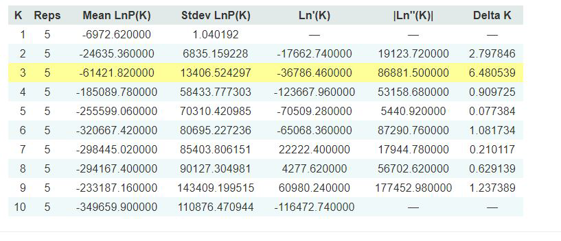
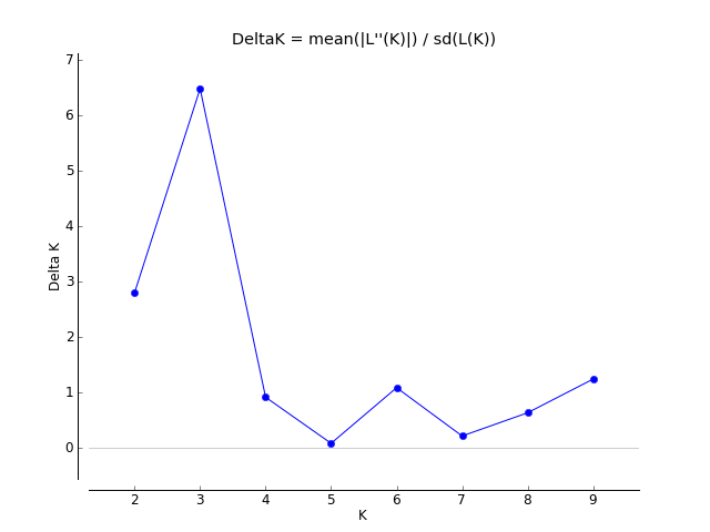
The Evanno table highlights the significant k value estimated for this genotype data (see figure below). For this tutorial data set, the estimated k is 3 subpopulations, which is also supported by the Delta K plot where a clear peak is seen at K = 3.
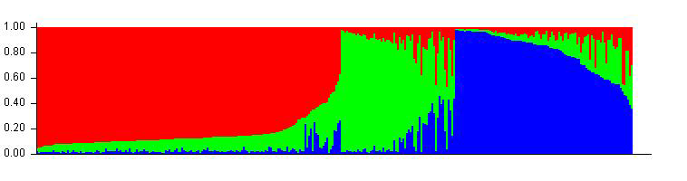
Therefore, the correct bar plot with the correct number of sub-populations (k = 3) can be plotted by following the steps shown in Step 1.4.
Thank you for reading this tutorial. If you have any questions or comments, please let me know by email.
Happy Structure-ing ![]()
Bibliography
Pritchard, Jonathan K., William Wen, and Daniel Falush. “Documentation for STRUCTURE software: Version 2.” (2003).
Earl, Dent A. “STRUCTURE HARVESTER: a website and program for visualizing STRUCTURE output and implementing the Evanno method.” Conservation Genetics Resources 4.2 (2012): 359–361.
Leave a comment